Grid Search Tuning

In this article, will cover the following four points:

Overview of Grid Search, and Cross Validation
Show how easy it is to run Grid Search model tuning in Spark
Provide a compelling reason to use ML Pipelines in our daily work
Highlight the advantages of using Spark, and sparklyr, for model tuning

Grid Search

The main goal of hyper-parameter tuning is to find the ideal set of model parameter values. For example, finding out the ideal number of trees to use for a model. We use model tuning to try several, and increasing values. That will tell us at what point a increasing the number of trees does not improve the model’s performance.

In Grid Search, we provide a provide a set of specific parameters, and specific values to test for each parameter. The total number of combinations will be the product of all the specific values of each parameter.

For example, suppose we are going to try two parameters. For the first parameter we provide 5 values to try, and for the second parameter we provide 10 values to try. The total number of combinations will be 50. The number of combinations grows quickly the more parameters we use. Adding a third parameter, with only 2 values, will mean that the number of combinations would double to 100 (5x10x2).

The model tuning returns a performance metric for each combination. We can compare the results, and decide which model to use.

In Spark, we use an ML Pipeline, and a list of the parameters and the values to try (Grid). We also specify the metric it should use to measure performance (See Figure 1). Spark will then take care of figuring out the combinations, and fits the corresponding models.

flowchart LR
  subgraph id1 [ ]
    subgraph id2 [ ]
      subgraph id3 [ML Pipeline]
        d[Prepare] --> m[Model]
      end
      subgraph id4 [Grid Search Tuning]
        m --> gv[Grid]
        gv-- Combo 1 -->ft1[Fit Models]
        ft1 --> ev1[Metric]
        gv-- Combo 2 -->ft2[Fit Models]
        ft2 --> ev2[Metric]     
        gv-- Combo 3 -->ft3[Fit Models]
        ft3 --> ev3[Metric]  
        gv-- Combo n -->ft4[Fit Models]
        ft4 --> ev4[Metric]          
      end
    end
  end
  style id1 fill:#eee,stroke:#eee
  style id2 fill:#eee,stroke:#eee
  style d fill:#99ccff,stroke#666
  style m fill:#99ffcc,stroke:#666
  style gv fill:#ffcc99,stroke:#666
  style ft1 fill:#ccff99,stroke:#666
  style ft2 fill:#ccff99,stroke:#666
  style ft3 fill:#ccff99,stroke:#666
  style ft4 fill:#ccff99,stroke:#666

Figure 1: Grid Search Tuning in Spark

Cross Validation

In Cross Validation, multiple models are fitted with the same combination of parameters. The difference is the data used for training, and validation. These are called folds. The training data, and the validation data is different for each fold, that is called re-sampling.

The model is fitted with the current fold’s training data, and then it is evaluated using the validation data. The average of the evaluation results become the official metric value of the combination of parameters. Figure 2, is a “zoomed” look of what happens inside Fit Models of Figure 1.

The total number of models, will be the total number of combinations times the number of folds. For example, if we use 3 parameters, with 5 values each, that would be 125 combinations. If tuning with 3 folds, Cross Validation will fit, and validate, a total of 375 models.

In Spark, running the 375 discrete models can be distributed across the entire cluster, thus significantly reducing the amount of time we would have to wait to see the results.

flowchart LR
  subgraph id1 [ ]
    subgraph id2 [ ]
      gv[Grid] -- Combo n -->re[Resample]
      re -- Fold 1 --> ft1[Fit]
      subgraph id4 [Fit Models with Cross Validation]
        re -- Fold 2 --> ft2[Fit]
        re -- Fold 3 --> ft3[Fit]
        ft1 --> ev1[Evaluate]
        ft2 --> ev2[Evaluate]     
        ft3 --> ev3[Evaluate]  
        ev1 --> eva[Avgerage]
        ev2 --> eva
        ev3 --> eva
      end
      eva --> mt[Metric]
    end
  end
  style id1 fill:#eee,stroke:#eee
  style id4 fill:#ccff99,stroke:#666
  style gv fill:#ffcc99,stroke:#666
  style ft1 fill:#ccffff,stroke:#666
  style ft2 fill:#ccffff,stroke:#666
  style ft3 fill:#ccffff,stroke:#666
  style re fill:#ffccff,stroke:#666
  style ev1 fill:#ffff99,stroke:#666
  style ev2 fill:#ffff99,stroke:#666
  style ev3 fill:#ffff99,stroke:#666
  style eva fill:#ffff66,stroke:#666

Figure 2: Cross Validation in Spark

Reproducing “Tuning Text Analysis” in Spark

In this article, we will reproduce the Grid Search tuning example found in the tune package’s website: Tuning Text Analysis. That example analyzes Amazon’s Fine Food Reviews text data. The goal is to tune the model using the exact same tuning parameters, and values, that were used in the tune’s website example.

Tip

This article builds on the knowledge of two previous articles, Text Modeling and Intro to Model Tuning. We encourage you to familiarize yourself with the concepts and code from those articles.

Spark and Data Setup

For this example, we will start a local Spark session, and then copy the Fine Food Reviews data to it. For more information about the data, please see the Data section of the Text Modeling article.

library(sparklyr)
library(modeldata)

data("small_fine_foods")

sc <- spark_connect(master = "local", version = "3.3")

sff_training_data <- copy_to(sc, training_data)
sff_testing_data <- copy_to(sc, testing_data)

ML Pipeline

As mentioned before, the data preparation and modeling in Text Modeling are based on the same example from the tune website’s article. The recipe steps, and parsnip model are recreated with Feature Transformers, and an ML model respectively.

Unlike tidymodels, there is no need to “pre-define” the arguments that will need tuning. At execution, Spark will automatically override the parameters specified in the grid. This means that it doesn’t matter that we use the exact same code for developing, and tuning the pipeline. We can literally copy-paste, and run the resulting pipeline code from Text Modeling.

sff_pipeline <- ml_pipeline(sc) %>% 
  ft_tokenizer(
    input_col = "review",
    output_col = "word_list"
  ) %>% 
  ft_stop_words_remover(
    input_col = "word_list", 
    output_col = "wo_stop_words"
    ) %>% 
  ft_hashing_tf(
    input_col = "wo_stop_words", 
    output_col = "hashed_features", 
    binary = TRUE, 
    num_features = 1024
    ) %>%
  ft_normalizer(
    input_col = "hashed_features", 
    output_col = "normal_features"
    ) %>% 
  ft_r_formula(score ~ normal_features) %>% 
  ml_logistic_regression()

sff_pipeline
#> Pipeline (Estimator) with 6 stages
#> <pipeline__1e8eb529_63ad_4182_b716_a32aa659c037> 
#>   Stages 
#>   |--1 Tokenizer (Transformer)
#>   |    <tokenizer__da641107_67cf_46bc_9d9b_075f5beb3dc7> 
#>   |     (Parameters -- Column Names)
#>   |      input_col: review
#>   |      output_col: word_list
#>   |--2 StopWordsRemover (Transformer)
#>   |    <stop_words_remover__24642e4c_01bf_48d4_b1d2_e3d439bdcdf6> 
#>   |     (Parameters -- Column Names)
#>   |      input_col: word_list
#>   |      output_col: wo_stop_words
#>   |--3 HashingTF (Transformer)
#>   |    <hashing_tf__bd5aebaa_864d_4ece_97e1_30fa0bbc515a> 
#>   |     (Parameters -- Column Names)
#>   |      input_col: wo_stop_words
#>   |      output_col: hashed_features
#>   |--4 Normalizer (Transformer)
#>   |    <normalizer__fd807e7a_0a8e_490f_b554_a19329337637> 
#>   |     (Parameters -- Column Names)
#>   |      input_col: hashed_features
#>   |      output_col: normal_features
#>   |--5 RFormula (Estimator)
#>   |    <r_formula__02516e56_4219_4277_91d1_7e5c0f4574bd> 
#>   |     (Parameters -- Column Names)
#>   |      features_col: features
#>   |      label_col: label
#>   |     (Parameters)
#>   |      force_index_label: FALSE
#>   |      formula: score ~ normal_features
#>   |      handle_invalid: error
#>   |      stringIndexerOrderType: frequencyDesc
#>   |--6 LogisticRegression (Estimator)
#>   |    <logistic_regression__89201a87_4f60_4ad3_a84c_d8e982c0988d> 
#>   |     (Parameters -- Column Names)
#>   |      features_col: features
#>   |      label_col: label
#>   |      prediction_col: prediction
#>   |      probability_col: probability
#>   |      raw_prediction_col: rawPrediction
#>   |     (Parameters)
#>   |      aggregation_depth: 2
#>   |      elastic_net_param: 0
#>   |      family: auto
#>   |      fit_intercept: TRUE
#>   |      max_iter: 100
#>   |      maxBlockSizeInMB: 0
#>   |      reg_param: 0
#>   |      standardization: TRUE
#>   |      threshold: 0.5
#>   |      tol: 1e-06

It is also worth pointing out that in a”real life” exercise, sff_pipeline would probably already be loaded into our environment. That is because we just finished modeling and, decided to test to see if we could tune the model (See Figure 3). Spark can re-use the exact same ML Pipeline object for the cross validation step.

Grid

There is a big advantage to transforming, and modeling the data in a single ML Pipeline. It opens the door for Spark to also alter parameters used for data transformation, in addition to the model’s parameters. This means that we can include the parameters of the tokenization, cleaning, hashing, and normalization steps as possible candidates for the model tuning.

The Tuning Text Analysis article uses three tuning parameters. Two parameters are in the model, and one is in the hashing step. Here are the parameters, and how they map between tidymodels and sparklyr:

Parameter	`tidymodels`	`sparklyr`
Number of Terms to Hash	`num_terms`	`num_features`
Amount of regularization in the model	`penalty`	`elastic_net_param`
Proportion of pure vs ridge Lasso	`mixture`	`reg_param`

Using partial name matching, we map the parameters to the steps we want to tune:

hashing_ft will be the name of the list object containing the num_features values
logistic_regression will be the of the list object with the model parameters

For more about partial name matching, see in the Intro Model Tuning article. For the parameters values, we can copy the exact same values from the tune website

sff_grid <-  list(
    hashing_tf = list(
      num_features = 2^c(8, 10, 12)  
    ),
    logistic_regression = list(
      elastic_net_param = 10^seq(-3, 0, length = 20), 
      reg_param = seq(0, 1, length = 5)    
    )
  )

sff_grid
#> $hashing_tf
#> $hashing_tf$num_features
#> [1]  256 1024 4096
#> 
#> 
#> $logistic_regression
#> $logistic_regression$elastic_net_param
#>  [1] 0.001000000 0.001438450 0.002069138 0.002976351 0.004281332 0.006158482
#>  [7] 0.008858668 0.012742750 0.018329807 0.026366509 0.037926902 0.054555948
#> [13] 0.078475997 0.112883789 0.162377674 0.233572147 0.335981829 0.483293024
#> [19] 0.695192796 1.000000000
#> 
#> $logistic_regression$reg_param
#> [1] 0.00 0.25 0.50 0.75 1.00

Evaluate

In the tune website’s article, ROC AUC is used to measure performance. The is the default metric of ml_binary_classification_evaluator() , so we only need to pass the connection variable to the evaluator function.

sff_evaluator <- ml_binary_classification_evaluator(sc)

Model Tuning

We will use ml_cross_validator() to prepare a tuning specification inside Spark. Spark will automatically create the parameter combinations when tuning the model. In this case, sff_grid contains three parameters:

num_features with 3 values
elastic_net_param with 20 values
reg_parm with 5 values

This means that there will be 300 combinations for the tuning parameters (3 x 20 x 5). Because we set the number of folds to 3 (num_folds), Spark will run a total of 900 models (3 x 300).

sff_cv <- ml_cross_validator(
  x = sc,
  estimator = sff_pipeline, 
  estimator_param_maps = sff_grid,
  evaluator = sff_evaluator,
  num_folds = 3,
  parallelism = 4,
  seed = 100
)

sff_cv
#> CrossValidator (Estimator)
#> <cross_validator__e3d09026_aa6f_4bf8_b1be_91dadd0c0b51> 
#>  (Parameters -- Tuning)
#>   estimator: Pipeline
#>              <pipeline__1e8eb529_63ad_4182_b716_a32aa659c037> 
#>   evaluator: BinaryClassificationEvaluator
#>              <binary_classification_evaluator__ca7cff64_45f7_4da6_9068_d0ec0c0f1de8> 
#>     with metric areaUnderROC 
#>   num_folds: 3 
#>   [Tuned over 300 hyperparameter sets]

Tip

We recommend to set the seed argument in order to increase reproducibility.

This is the step that will take the longest time. The ml_fit() function will run the 900 models using the training data. There is no need to pre-prepare the re-sampling folds, Spark will take care of that.

sff_model <- ml_fit(
  x = sff_cv, 
  dataset = sff_training_data
  )

Metrics

We can now extract the metrics from sff_model using ml_validation_metrics(). The ROC AUC values will be in a column called areaUnderROC. We can then take a look at the best performing models using dplyr.

sff_metrics <- ml_validation_metrics(sff_model)

library(dplyr)

sff_metrics %>% 
  arrange(desc(areaUnderROC)) %>% 
  head()
#>   areaUnderROC elastic_net_param_1 reg_param_1 num_features_2
#> 1    0.7858727          0.05455595        0.25           4096
#> 2    0.7847232          0.02636651        0.50           4096
#> 3    0.7835850          0.01832981        0.75           4096
#> 4    0.7830411          0.01832981        0.50           4096
#> 5    0.7830230          0.03792690        0.25           4096
#> 6    0.7828651          0.01274275        0.75           4096

We will now plot the results. We will match the approach used in the Grid Search section of the Tuning Text Analysis article.

library(ggplot2)

sff_metrics %>% 
  mutate(reg_param_1 = as.factor(reg_param_1)) %>% 
  ggplot(aes(
    x = elastic_net_param_1, 
    y = areaUnderROC, 
    color = reg_param_1
    )) +
  geom_line() +
  geom_point(size = 0.5) +
  scale_x_continuous(trans = "log10") +
  facet_wrap(~ num_features_2) +
  theme_light(base_size = 9)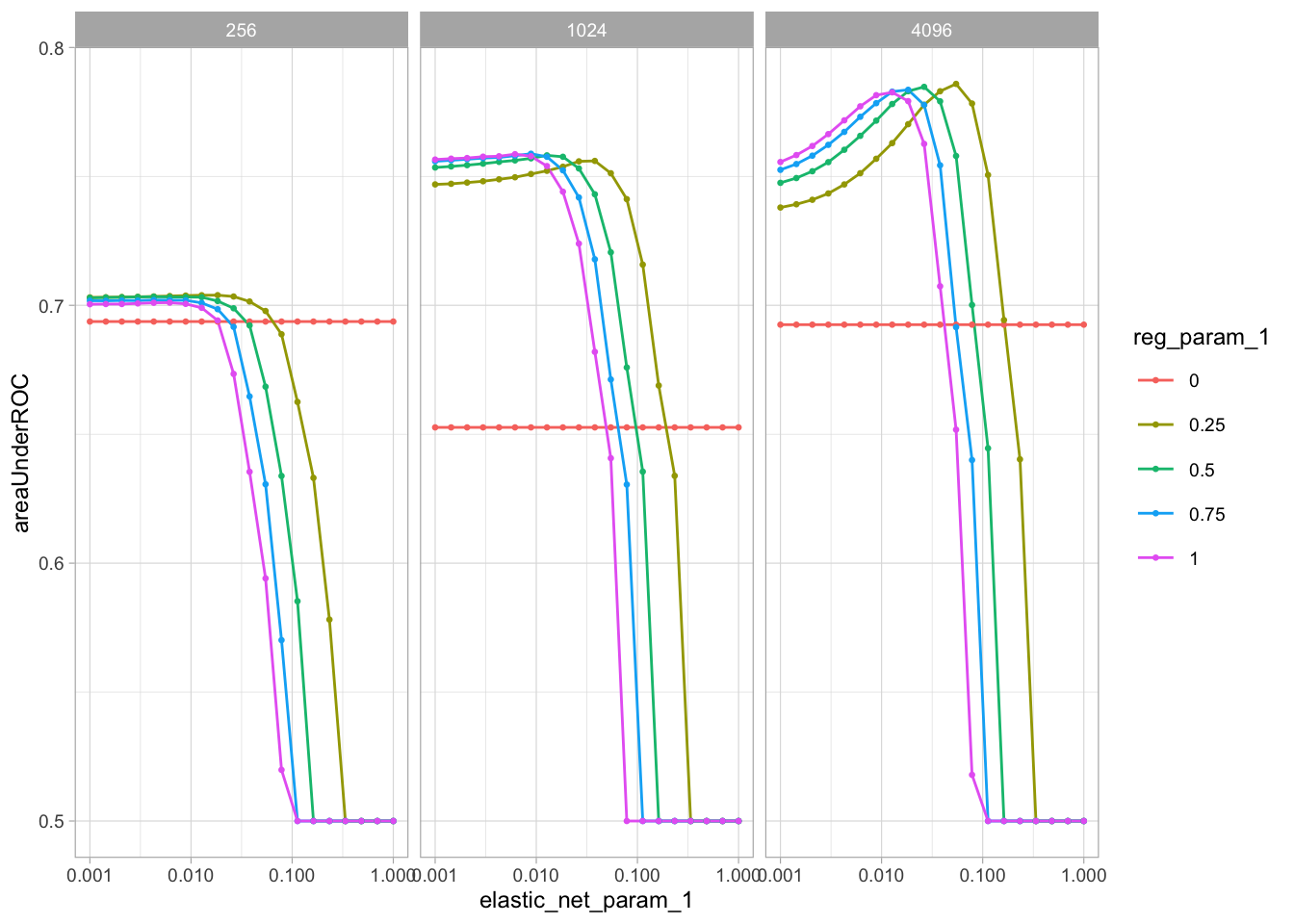

In the plot, we can see the effects of the three parameters, and the values that look to be the best. These effects are very similar to the original tune’s website article.

Model selection

We can create a new ML Pipeline using the same code as the original pipeline. We only need to change the 3 parameters values, with values that performed best.

new_sff_pipeline <- ml_pipeline(sc) %>% 
  ft_tokenizer(
    input_col = "review",
    output_col = "word_list"
  ) %>% 
  ft_stop_words_remover(
    input_col = "word_list", 
    output_col = "wo_stop_words"
    ) %>% 
  ft_hashing_tf(
    input_col = "wo_stop_words", 
    output_col = "hashed_features", 
    binary = TRUE, 
    num_features = 4096      
    ) %>%
  ft_normalizer(
    input_col = "hashed_features", 
    output_col = "normal_features"
    ) %>% 
  ft_r_formula(score ~ normal_features) %>% 
  ml_logistic_regression(
    elastic_net_param = 0.05,
    reg_param = 0.25  
    )

Now, we create a final model using the new ML Pipeline.

new_sff_fitted <- new_sff_pipeline %>% 
  ml_fit(sff_training_data)

The test data set is now used to confirm that the performance gains hold. We use it to run predictions with the new ML Pipeline Model.

new_sff_fitted %>% 
  ml_transform(sff_testing_data) %>% 
  ml_metrics_binary()
#> # A tibble: 2 × 3
#>   .metric .estimator .estimate
#>   <chr>   <chr>          <dbl>
#> 1 roc_auc binary         0.783
#> 2 pr_auc  binary         0.653

Benefits of ML Pipelines for everyday work

In the previous section, the metrics show an increase performance compared to the model in the Text Modeling article.

The gains in performance were easy to obtain. We literally took the exact same pipeline we used in developing the model, and ran it through the tuning process. All we had to create was a simple grid, and a provide the metric function.

This highlights an advantage of using ML Pipelines. Because transitioning from modeling to tuning in Spark, will be a simple operation. An operation that has the potential to yield great benefits, with little cost of effort. (Figure 3)

flowchart LR
  subgraph id1 [ ]
  subgraph id2 [ ]
    subgraph si [ML Pipeline]
      dm[Data prep<br> & model] 
    end
    dm -- Development<br>cycle --> t[Test] 
    t --> dm
    t -- Selected<br>ML Pipeline  --> tn[Tune]
    gm[Grid & Metric] --> tn
    subgraph sp [ML Pipeline]
      fm[Final model] 
    end
    tn -- Best<br>parameters --> fm
  end
  end
  style t fill:#ffcc00,stroke:#000
  style tn fill:#ffcc99,stroke:#000
  style dm fill:#ffff99,stroke:#000
  style fm fill:#ffff99,stroke:#000
  style id1 fill:#eee,stroke:#eee
  style id2 fill:#eee,stroke:#eee
  style gm fill:#fff,stroke:#000

Figure 3: Developing models with ML Pipelines

Accelerate model tuning with Spark

As highlighter in the previous section, Spark, and sparklyr, provide an easy way to go from exploration, to modeling, and tuning. Even without a “formal” Spark cluster, it is possible to take advantage of these capabilities right from our personal computer.

If we add an actual cluster to the mix, the advantage of using Spark raises dramatically. Usually, we talk about Spark for “big data” analysis, but in this case, we can leverage it to “parallelize” hundreds of models across multiple machines. The ability to distribute the models across the cluster will cut down the tuning processing time (Figure 4). The resources available to the cluster, and the given Spark session, will also determine the the amount of time saved. There is really no other open-source technology that is capable of this.

classDiagram
  class Driver {
  }
  class Node1{
    Job 1 - Model 1
    Job 2 - Model 2
    Job 3 - Model 3
    Job 4 - Model 4    
  }
  class Node2{
    Job 1 - Model 5
    Job 2 - Model 6
    Job 3 - Model 7
    Job 4 - Model 8       
  }
  class Node3{
    Job 1 - Model 9
    Job 2 - Model 10
    Job 3 - Model 11
    Job 4 - Model 12      
  }  
  class Node4{
    Job 1 - Model 13
    Job 2 - Model 14
    Job 3 - Model 15
    Job 4 - Model 16      
  }    
  Driver --> Node1
  Driver --> Node2
  Driver --> Node3
  Driver --> Node4

Figure 4: Model tuning in a Spark cluster